Income, Sleepiness, and Depression

Question

Does adding household income improve our ability to predict depression beyond daytime sleepiness alone?

Key Finding

Both daytime sleepiness and household income independently predict depression. A one-level increase in daytime sleepiness was associated with nearly double the odds of screening positive for depression (OR = 1.95). Higher income was associated with lower odds (OR = 0.77 per unit increase in the income-to-poverty ratio). Adding income to the sleepiness model improved fit modestly (Pseudo R² from 0.080 to 0.099), and the sleepiness coefficient barely changed — suggesting the two variables are largely independent predictors rather than one explaining the other.

Initial Hypothesis

Yes — income is a known social determinant of mental health, and I expected it to add predictive value beyond sleepiness, though sleepiness would remain the stronger predictor.

Dataset

NHANES 2017–2018, National Center for Health Statistics.

• SLQ — Sleep Disorders questionnaire. The key variable is SLQ120: “In the past month, how often did you feel excessively or overly sleepy during the day?” Responses are ordinal: 0 = Never, 1 = Rarely (1×/month), 2 = Sometimes (2–4×/month), 3 = Often (5–15×/month), 4 = Almost Always (16–30×/month).
• DPQ — Patient Health Questionnaire (PHQ-9) depression screener, same instrument as Investigation 001 and Investigation 002.
• DEMO — Demographics file. The key variable is INDFMPIR: the ratio of family income to the federal poverty guideline, ranging from 0 to 5 (where 5 indicates income at or above 5× the poverty line).

View the analysis notebook on GitHub

Cleaning

Three datasets were merged on respondent ID (SEQN): the Sleep Disorders questionnaire (SLQ), the depression screener (DPQ), and the Demographics file (DEMO). All three joins were inner joins, keeping only participants with data in all three sources. Because the goal is to compare three models — depression predicted by sleepiness alone, by income alone, and by both together — all models must be fit on the same sample to allow fair comparison.

NHANES codes refused and “don’t know” responses as 7 or 9. These were replaced with missing values in SLQ120 and all nine PHQ-9 items (DPQ010–DPQ090), and rows missing any of these variables were dropped. INDFMPIR required no special recoding; values near zero represent genuine near-zero income, and missing values (1,231 participants, ~13% of the demographics file) were handled by the row-drop step.

The final analysis sample contains 4,433 participants, down from 5,533 after the initial SLQ/DPQ merge. The ~1,100 person reduction is due primarily to missing income data. Participants who did not report income may differ systematically from those who did — this is noted as a limitation below.

The PHQ-9 total score was calculated as the sum of DPQ010–DPQ090 (range 0–27). A binary depression variable was created using the standard clinical cutoff: PHQ-9 ≥ 10 = depressed (1), PHQ-9 < 10 = not depressed (0). This produced an imbalanced sample: 392 depressed (9%) and 4,041 not depressed (91%).

Analysis

Introduction

Investigations 001 and 002 explored the relationship between sleep and depression using correlation and linear regression. Investigation 002 found that daytime sleepiness alone explained about 16% of the variance in PHQ-9 scores — a meaningful but modest result. This investigation asks whether adding a socioeconomic factor, household income, improves our ability to predict depression.

The outcome variable changes here in an important way. Rather than predicting a continuous PHQ-9 score, we predict whether a person screens positive for depression — defined as a PHQ-9 score of 10 or higher, the standard clinical cutoff for moderate-to-severe depression. Because the outcome is now binary, we use logistic regression instead of linear regression. Logistic regression is the appropriate model when you are predicting a yes/no outcome, and it produces odds ratios that make the results straightforward to interpret.

We build three models: depression predicted by sleepiness alone, depression predicted by income alone, and depression predicted by both together. Fitting all three on the same sample lets us compare the individual predictive power of each variable and observe whether they behave as largely independent effects or whether one attenuates the other when they share a model.

Stage 1 — Sleepiness Only

	Value
Coefficient (SLQ120)	0.695
Odds Ratio	2.00
95% CI	[1.82, 2.21]
Pseudo R²	0.080
p-value	<0.0001

Daytime sleepiness is a highly significant predictor of depression. Each one-level increase on the sleepiness scale is associated with approximately double the odds of screening positive for depression (OR = 2.00, 95% CI [1.82, 2.21]). The confidence interval sits well above 1.0, leaving little uncertainty about the direction of the association.

The Pseudo R² of 0.080 indicates a moderate fit by McFadden’s standards (0.05–0.10). This is not directly comparable to the R² from Investigation 002 — McFadden’s R² tends to run much lower than OLS R² even for well-fitting models, so the two numbers should not be compared directly. McFadden’s R² measures improvement over a model containing only an intercept.

Stage 2 — Income Only and Combined Model

Model 2: Depression ~ Income

	Value
Coefficient (INDFMPIR)	-0.289
Odds Ratio	0.75
95% CI	[0.70, 0.81]
Pseudo R²	0.025
p-value	<0.0001

Income is a statistically significant predictor of depression, but a weaker standalone predictor than sleepiness. Each one-unit increase in the income-to-poverty ratio is associated with 25% lower odds of screening positive for depression (OR = 0.75). The Pseudo R² of 0.025 is substantially lower than the 0.080 from the sleepiness-only model, confirming that sleepiness carries more predictive information on its own.

Model 3: Depression ~ Sleepiness + Income

	Coefficient	Odds Ratio	95% CI
SLQ120	0.670	1.95	[1.77, 2.16]
INDFMPIR	-0.261	0.77	[0.72, 0.83]

Pseudo R² = 0.099

Adding income improves model fit modestly, with the Pseudo R² rising from 0.080 to 0.099. Both predictors remain highly significant and their confidence intervals stay well clear of 1.0. Each coefficient represents the effect of that variable holding the other constant — so the sleepiness odds ratio of 1.95 reflects the effect of sleepiness among people at the same income level, and vice versa.

The sleepiness odds ratio dropped only slightly when income was added, from 2.00 to 1.95 — a 5% attenuation. This small change suggests that sleepiness and income are largely independent predictors of depression. Income accounts for a tiny portion of the sleepiness effect but does not explain it away.

Stage 3 — Model Evaluation

ROC Curve and AUC

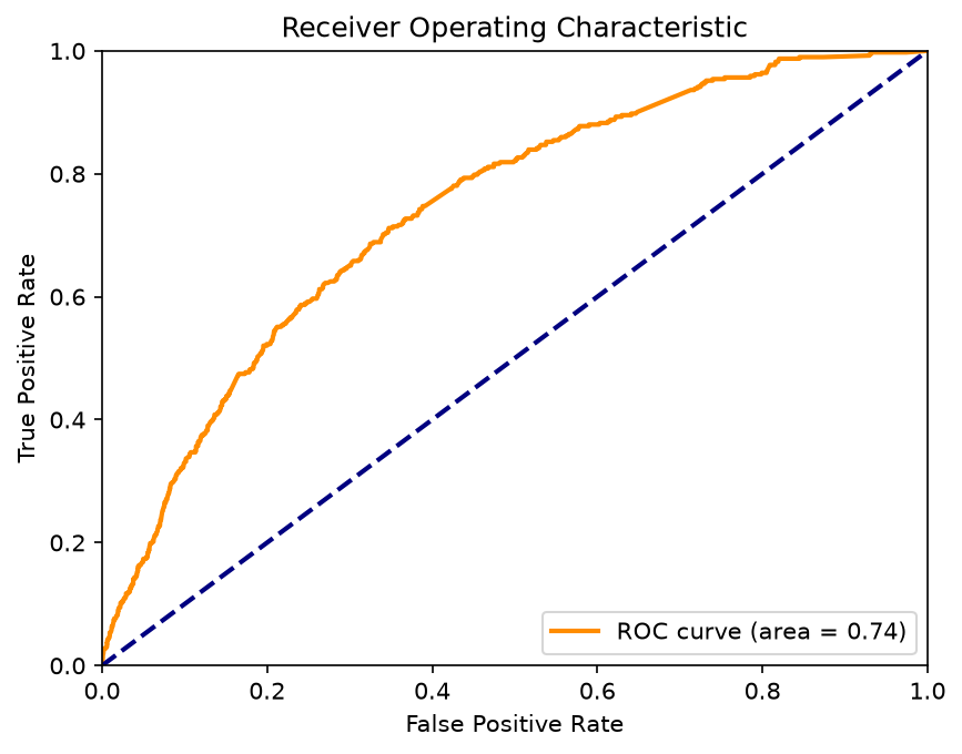
The AUC of 0.74 means the model correctly ranks a randomly chosen depressed person above a randomly chosen non-depressed person 74% of the time. This falls in the range often interpreted as “acceptable” discrimination (0.70–0.80) — meaningfully better than random chance (0.50), but short of the “excellent” threshold (0.80+) that would be expected of a clinical screening tool.

Confusion Matrix

At the standard classification threshold of 0.50, the model predicted nobody as depressed — all 4,433 participants were classified as not depressed. This is a direct consequence of class imbalance. With only 9% of the sample screening positive, the model learned that predicting “not depressed” for everyone minimizes error at that threshold. The confusion matrix result does not mean the model learned nothing; it means the 0.50 threshold is the wrong threshold for this data.

Predicted Probabilities

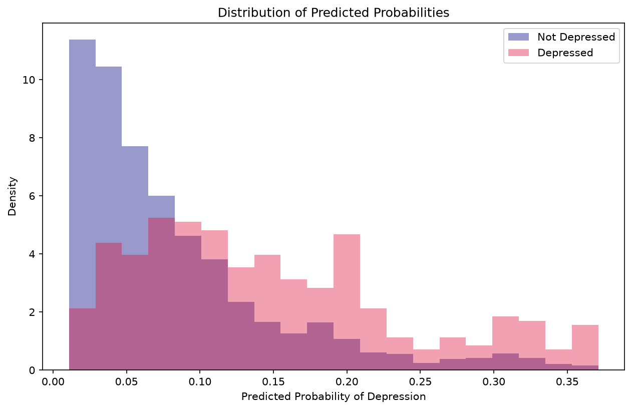
The density plot shows what the model actually learned. The not-depressed group (blue) is concentrated at very low predicted probabilities, mostly below 0.05. The depressed group (red) is flatter and extends further right, with meaningful density out to 0.35. The model assigns higher probabilities to people who are actually depressed — it discriminates — but the two distributions overlap substantially in the 0.05–0.20 range, and no one receives a predicted probability above 0.38. This explains why the 0.50 threshold fails: the model is uncertain, not wrong. A lower threshold would begin to separate the groups at the cost of more false positives.

Limitations

Income ceiling. INDFMPIR is capped at 5.0 — anyone earning above five times the poverty line receives the same value regardless of actual income. This means the model cannot distinguish between a household at 5× and one at 20× the poverty line, and cannot estimate whether depression risk continues to fall at higher income levels. The most practically important variation in this variable likely occurs in the lower range (0–3), where crossing the poverty line has real material consequences, so the ceiling probably has limited impact on the main findings.

Correlation, not causation. This analysis cannot determine the direction of any causal relationship. Depression may cause sleepiness — through disrupted sleep, or through medications used to treat depression that carry sedation as a side effect. Low income may cause depression through the chronic stress and limited options that come with financial hardship. And both relationships may be driven by a third variable not included in the model. Chronic illness is a plausible candidate: it can limit employment and reduce income, disrupt sleep and cause fatigue, and produce a sense of hopelessness that contributes to depression. The associations we found are real, but their causal structure cannot be determined from this data.

Missing income data. Approximately 1,100 participants were dropped due to missing INDFMPIR values. People who do not report income may differ systematically from those who do — for example, individuals between jobs may be uncertain what to report, and periods of unemployment are themselves a risk factor for depression. If the people we dropped were more likely to be depressed than those we kept, our results may underestimate the true relationship between income and depression in the full population.

Class imbalance. Only 9% of the analysis sample screened positive for depression. This made standard classification at a 0.50 threshold uninformative — the model predicted no one as depressed. The AUC and predicted probability distribution are more honest summaries of model performance in this setting. Approaches such as threshold adjustment, oversampling the minority class, or class-weighted models could improve classification performance but were beyond the scope of this investigation.

Two predictors. This model uses only two predictors. Depression is influenced by many biological, psychological, and social factors not captured here — chronic illness, social support, life events, genetics, and many others. This model is a starting point, not a complete account.

If I Had More Time

• Address class imbalance directly. With only 9% of the sample screening positive for depression, the model never predicted anyone as depressed at the standard 0.50 threshold. Techniques such as adjusting the classification threshold using the ROC curve, oversampling the minority class (SMOTE), or fitting a class-weighted logistic regression would produce a model that actually classifies people — and would make the confusion matrix a useful diagnostic rather than a trivial result.
• Add covariates. Age, sex, BMI, chronic illness status, and marital status are all plausible confounders. A richer model would help isolate the independent contributions of sleepiness and income.
• Examine the mediation hypothesis more rigorously. The 5% attenuation of the sleepiness coefficient when income was added is suggestive but not conclusive. A formal mediation analysis (e.g., using the pingouin or statsmodels mediation tools) would test whether income partially mediates the sleepiness-depression relationship — or whether sleepiness mediates the income-depression relationship.
• Revisit the income variable. INDFMPIR measures income relative to the federal poverty guideline, which accounts for household size but not financial obligations. Two households at the same ratio can experience very different financial pressure depending on eldercare responsibilities, dependent children in college, or retirement savings needs. A future investigation could explore whether financial stress measures — rather than raw income ratios — predict depression more strongly.

Next Investigation

004 — TBD